
Urban sensing: quantifying the sensing power of vehicle fleets
Introduction
Smart cities are increasingly being equipped with sensors measuring a variety of quantities indicative of the quality of the urban enviroment: air pollution, traffic congestion, air temperature, humidity, road quality, pedestrian density, parking spot occupancy, Wi-Fi accessibility, etc. All these measurements will fuel advanced urban analytics, and become a routine component in urban planning, policy making, and management.
However, the city-wide deployment of sensors has limited spatial coverage and comes at a significant cost, and the question of their optimal placement arises naturally. As a solution, the “drive-by” paradigm has been recently proposed, whereby sensors are installed on third-party vehicles “scanning” the city. While most of the research on drive-by sensing has focused on engineering aspects, the key question of how many vehicles are required to adequately scan a city remained unanswered until recently. The answer intuitively depends on the mobility patterns of the vehicles in question. Among many candidates for the vehicle fleets, such as private cars, buses, and taxis, taxis are the natural choice for deploying the sensors as they are pervasive in the city and do not follow fixed routes. Is it possible to find out whether attaching sensors to taxi vehicles is a good idea? This is what we are going to do in this post.
Why is it important?
If we discover that a small number of taxis covers a large portion of the city, attaching sensors to those taxis could provide a cheap way for monitoring the various quantities mentioned in the introduction. In this post, we define a measure of this “covering” and discuss its analytic description, which agrees surprisingly well with empirical data from a ride sharing company called GG based in Yerevan. We will follow the arguments described in a recent paper from the MIT Senseable Lab to demonstrate the suprisingly huge potential of this method: just 30 randomly chosen taxi vehicles (less than 1% of the entire fleet) during a typical day cover on average more than a third of Yerevan city and almost 70% of the centrally located districts (Kentron, Ajapnyak, Kanaker-Zeytun, Nork-Marash)! This has huge implications for smart city projects as it demonstrates that drive-by sensing can be readily implemented in real projects at a relatively small cost.
How to measure urban sensing?
In order for a vehicle fleet to scan as large a portion of the urban street network as possible, a dense exploration of what the authors call the city’s spatio-temporal “volume” is required. The extent to which a vehicle fleet does this is called its sensing power.
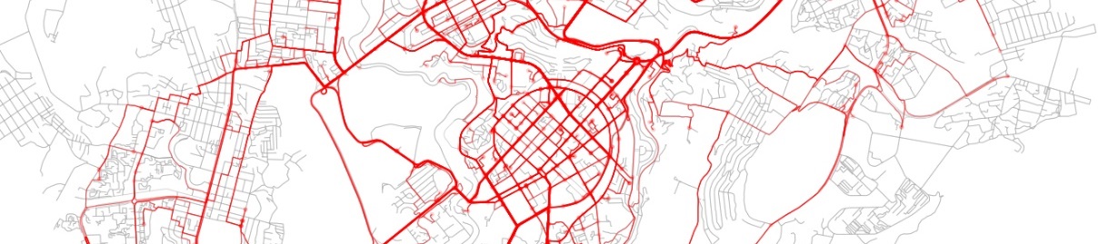
Imagine a fleet of sensor-equipped vehicles \(\mathcal{V}\) moving in a city, scanning its street network \(S\) during a reference period \(\mathcal{T}\). Below you can see such a fleet of randomly chosen 30 taxis traversing the streets of Yerevan:
We represent the nodes of the street network \(S\) as potential pick-up and drop-off locations for the vehicles. Since we are going to work with street segments, we convert the set of GPS coordinates of a given vehicle to a trajectory \(T_{r}\), defined as a sequence of street segments \(T_{r} = (S_{i_1} , S_{i_2} , . . . )\). In order to achieve this, we need to match the taxi trajectories to the OpenStreetMap driving network segments. However, this is not an easy task, since a naive projection to the closest road segment yields incorrect results. Fortunately, this problem has been solved in this paper, which builds a Hidden Markov Model for identifying the most probable street network path, given a sequence of GPS points.
In order to measure the sensing power of a fleet, we quantify it as its covering fraction \(\langle C\rangle\), defined in the paper as the average fraction of street segments in \(S\) that are “covered” or sensed by a taxi during time period \(\mathcal{T}\) , assuming that \(N_{V}\) vehicles are selected uniformly at random from the vehicle fleet \(\mathcal{V}\).
What we want is an understanding of how the sensing power of a vehicle fleet in a city changes as a function of the size of the fleet.
Can we simulate the taxi movements?
To model the taxis’ movements, the paper introduces the taxi-drive process. The model makes very simple (and wrong) assumptions:
- that taxis travel to randomly chosen destinations via shortest paths, with ties between multiple shortest paths broken at random.
- Once a destination is reached, another destination is chosen, again at random, and the process repeats.
- To reflect heterogeneities in real taxi trajectories, destinations are not selected uniformly at random. Instead, already visited nodes are chosen preferentially: The probability \(q_{n}(t)\) of selecting a node \(n\) is proportional to \(1+v_{n}^{\beta}(t)\), where \(v_{n}(t)\) is the total number of times node \(n\) has been visited at during the time interval \((t_{start}, t)\) and \(\beta\) is a city-specific parameter to be tweaked. This “preferential attachment” mechanism, colloquially known as rich-get-richer effect and discussed mainly within the context of wealth distribution and tie formation in social networks, has been shown to capture the statistical properties of human mobility and, as it turns out, also captures those of taxis.
We first calculate the street segment popularities \(p_{i}\), the relative frequency each street segment in the city is traversed by the vehicles in the fleet \(\mathcal{V}\) during \(\mathcal{T}\) (the \(p_{i}\) sum to 1) from the GG taxi data (spoiler: we are going to use the \(p_{i}\) to compute our target \(\langle C\rangle\)). Then, we run the simulation of the taxi-drive process with the same fleet size and the same number of trips for each vehicle. We discover that, despite the unrealistic assumptions in the model, the taxi-drive process captures quite well the statistical properties of real taxis’ trajectories.
In particular, the simulation produces surprisingly realistic distributions of segment popularities \(p_{i}\), in agreement with that obtained from the GG data:
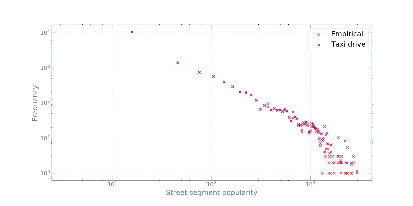
As one might expect from a preferential attachment mechanism, the distributions are heavy-tailed and closely follow Zipf’s law. This good agreement between the model and the data is rather surprising. One might expect that the simplistic assumptions in the taxi-drive model miss many important factors in the real world, such as variations in street-segment lengths and driving speeds, the spatial arranagement of attractive destinations specific to a city, human-routing decisions, as well as heterogeneities in passenger-pickup and -dropoff times and locations. However, the results show that, at the macro level of segment popularity distributions, these complexities are irrelevant. Moreover, the original paper finds this agreement to be true across many cities varying in size and continent.
Analytic derivation of \(\langle C_{N_V}\rangle\)
Having computed the segment popularities \(p_{i}\), we now proceed to estimating the sensing power \(\langle C_{N_V}\rangle\) analytically by recognizing the connection with the urn problem in probability theory (this is why knowledge of basic probability theory is so useful!). The street segments are considered as “bins” into which “balls” are placed every time a taxi vehicle traverses that street segment. Using the segment popularities \(p_{i}\) as the bin probabilities, we can derive the analytic expression for \(\langle C_{N_V}\rangle\).
As stated in the paper, given the nontrivial topology of \(S\) and the non-Markovian nature of the taxi-drive process (this essentially means that the future does not only depend on the present - loosely speaking the Markov property - but on the past as well), it is difficult to solve for \(\langle C_{N_V}\rangle\) exactly. However, it is possible to derive a very good approximation.
As we will see in a bit, it is actually easier to first solve for the trip-level \(\langle C_{N_T}\rangle\) covered fraction — i.e., when \(N_T\), the total number of trips, is the dependent variable, so we begin the derivation with this simpler case; the vehicle-level expression for \(\langle C_{N_V}\rangle\) will then be trivial to obtain.
Imagine we have a set \(\mathcal{P}\) of taxi trajectories. We define a taxi trajectory \(T_r\) as a sequence of street segments \(T_{r} = (S_{i_1} , S_{i_2} , . . . )\). The trajectories can be those obtained from the empirical data or from the simulation - this is unimportant for now. Given \(\mathcal{P}\), our strategy for finding \(\langle C_{N_T}\rangle\) will be to imagine street segments as bins into which balls are added every time they are traversed by a trajectory from \(\mathcal{P}\). Note that, in contrast to the traditional urn problem, a random number of balls is placed at each time step, since taxis’ trajectories have random length.
Trajectories with unit length
Let \(L\) be the random length of a trajectory. The special case of \(L=1\) is trivial to solve, since it corresponds exactly to the classical case: drawing \(N_T\) trips at random from \(\mathcal{P}\) amounts to adding \(N_T\) balls into \(N_S\) bins, where \(N_S\) is the total number of street segments, and each bin is selected with probability \(p_i\). Let \(\vec{M}=(M1, M2, . . ., M_{N_S})\), where \(M_i\) is the number of balls in the \(i\)-th bin. It is well known that the \(M_i\) are multinomially distributed:
\(\vec{M} \sim \operatorname{Multi}\left(N_{T}, \vec{p}\right)\),
where \(\vec{p}=\left(p_{1}, p_{2}, \dots p_{N_{s}}\right)\). Now, since a street segment is considered covered during time period \(\mathcal{T}\) if it is traversed by at least one vehicle from \(\mathcal{V}\), the (random) fraction of street segments covered is
\(C=\frac{1}{N_{S}} \sum_{i=1}^{N_{S}} 1_{\left(M_{i} \geq 1\right)}\),
where \(1_A\) is the indicator function of event \(A\). The expectation of this fraction \(C\) is
\(\langle C\rangle_{\left(N_{T}, L=1\right)}=\frac{1}{N_{S}} \sum_{i=1}^{N_{S}} \mathbb{P}_{N_{T}}\left(M_{i} \geq 1\right)\).
Now the trick is to note that the number of balls in each bin is a binomial random variable \(M_{i} \sim B i\left(N_{T}, p_{i}\right)\). The survival function of the binomial distribution is \(\mathbb{P}\left(M_{i} \geq 1\right)=1-\left(1-p_{i}\right)^{N_{T}}\). Finally, we substitute this into the previous equation and obtain:
\(\langle C\rangle_{\left(N_{T}, L=1\right)}=1-\frac{1}{N_{S}} \sum_{i=1}^{N_{S}}\left(1-p_{i}\right)^{N_{T}}\).
Trajectories with fixed length
Trajectories of fixed (i.e., nonrandom) length \(L>1\) lead to spatial correlations between the counts \(M_i\) (note: in the classic urn problem, there is already a correlation among the \(M_i\), since their sum is constant and equal to the total number of balls placed). This is due to the fact that real trajectories are contiguous in space: a trajectory that covers a given segment cannot jump the neighbouring segments at a node, and has to cover one of the neighboring segments. Given the nontrivial topology of the street network \(S\), the correlations between bins are difficult to model (this would require working with the adjacency matrix of the street network \(S\)). To overcome this, the authors in the paper made the strong assumption that for \(N_{T} \gg 1\), the spatial correlations between bins are asymptotically zero. This assumption renders our task much more easier. We now imagine that adding a trajectory of length \(L\) is the same as if we add \(L\) balls into (not necessarily contiguous) bins chosen randomly according to \(p_i\). This means that choosing \(N_T\) trajectories of fixed length \(L\) from \(\mathcal{P}\) is equivalent to placing \(L \star N_T\) balls into \(N_S\) bins: \(\langle C\rangle_{\left(N_{T}, L_{f i x e d}\right)}=\langle C\rangle_{\left(N_{T} \star L, L=1\right)}\). Hence, the expected value of the coverage can be obtained by modifying the result obtained in the unit length case:
\(\langle C\rangle_{\left(N_{T}, L_{f i x e d}\right)}=1-\frac{1}{N_{S}} \sum_{i=1}^{N_{S}}\left(1-p_{i}\right)^{L * N_{T}}\).
The assumption that neighbouring street segments are spatially uncorellated is a gross simplification which essentially removes the spatial component from the model. However, as we will see in a bit, it produces results remarkably consistent with the data.
Trajectories of random lengths
Now, generalizing to random \(L\) is easy. Let \(S_{N_{T}}=\sum_{i=1}^{N_{T}} L_{i}\) be the number of segments covered by \(N_T\) trajectories. By the law of total expectation
\(\langle C\rangle_{\left(N_{T}, L\right)}=\sum_{n=0}^{\infty}\langle C\rangle_{\left(n, L_{f i x e d}\right)} \mathbb{P}\left(S_{N_{T}}=n\right)\),
where \(\langle C\rangle_{\left(n, L_{\text {fixed}}\right)}\) is given by the expression for fixed \(L\). Finding the probabilities \(\mathbb{P}\left(S_{N_{T}}=n\right)\) is trickier. We need to know the distribution of the trajectory lengths. In the paper, the authors show that \(L \sim L o g n o r m a l\left(\tilde{\mu}, \tilde{\sigma}^{2}\right)\). We confirm this finding on the GG vehicle trajectory lengths with fitting a longormal distribution to the trajectory lengths and finding \((\mu, \sigma,\langle L\rangle)=(3.00,0.86,27.80)\):
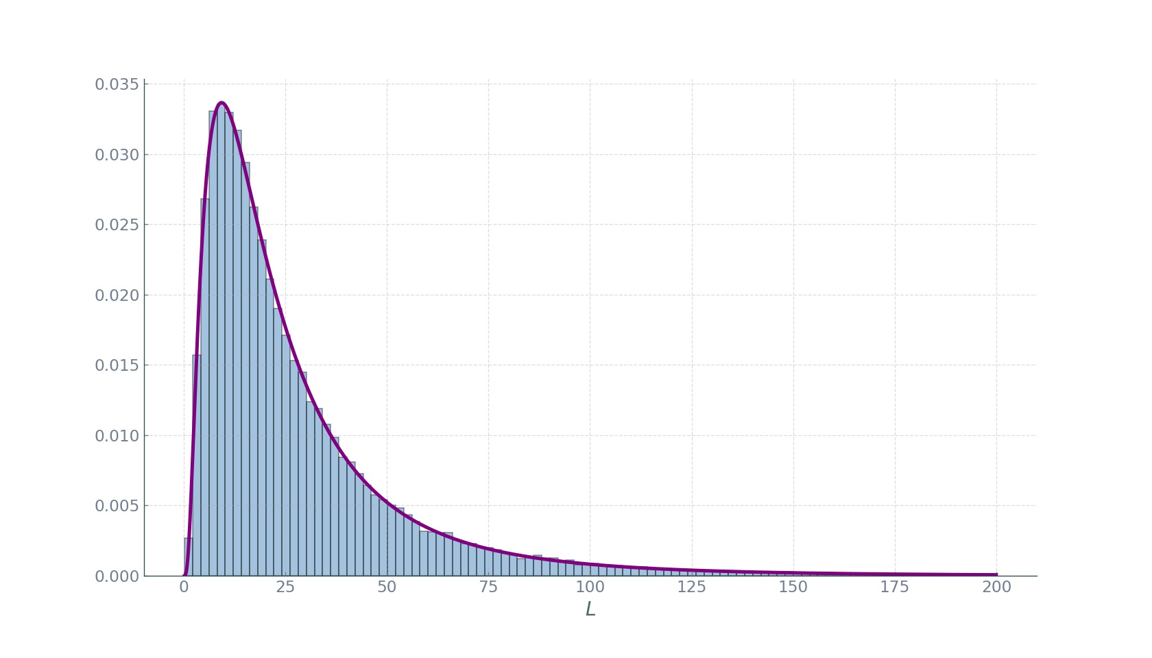
To remind again: \(L\) measures the number of segments covered by a vehicle, and not the distance of the trip. Further, it has been shown that the sum of lognormal random variables is itself approximately lognormal \(S_{N_{T}} \sim \operatorname{Lognormal}\left(\mu_{S,} \sigma_{S}^{2}\right)\) for some \(\mu_{S}\) and \(\sigma_{S}\). In order to choose appropriate \(\mu_{S}\) and \(\sigma_{S}\), the authors follow the Fenton-Wilkinson method in which \(\sigma_{S}^{2}=\ln \left(\frac{\exp \tilde{\sigma}^{2}-1}{N_{T}}+1\right)\) and \(\mu_{S}=\ln \left(N_{T} \exp (\tilde{\mu})\right)+\left(\tilde{\sigma}^{2}-\sigma_{S}^{2}\right) / 2\). Plugging into the lognormal pdf formula, we obtain
\(\mathbb{P}\left(S_{N_{T}}=n\right)=\frac{1}{n \sigma_{S} \sqrt{2 \pi}} \mathrm{e}^{-\frac{\left(\ln n-\mu_{S}\right)^{2}}{2 \sigma_{S}^{2}}}\).
And substituting this into the previous equation above, we obtain the nasty
\(\langle C\rangle_{\left(N_{T}, L\right)}=\frac{1}{N_{S} n \sigma_{S} \sqrt{2 \pi}} \sum_{n=0}^{\infty} \sum_{i=1}^{N_{S}}\left(1-\left(1-p_{i}\right)^{n}\right) \mathrm{e}^{-\frac{\left(\ln n-\mu_{S}\right)^{2}}{2 \sigma_{S}^{2}}}\).
This equation completely models the trip-level fraction \(\langle C\rangle_{\left(N_{T}, L\right)}\). However, a non-trivial thing to notice: the sum over \(n\) is dominated by its expectation, so we simplify matters by replacing \(n\) by its expected value \(\langle L\rangle \star N_{T}\). This gives us much simpler and nicer formula \(\left.\langle C\rangle_{\left(N_{T}, L\right)}=\langle C\rangle_{\left(N_{T}^{*}\right.}\langle L\rangle, L=1\right)\), or
\(\langle C\rangle_{N_{T}} \approx 1-\frac{1}{N_{S}} \sum_{i=1}^{N_{S}}\left(1-p_{i}\right)^{\langle L\rangle \star N_{T}}\).
Extension to vehicle level
As promised, now we do the final step of obtaining the fraction \(\langle C\rangle_{N_V}\) as a function of the number of vehicles. Let \(B\) be the random number of segments that a random taxi in \(\mathcal{V}\) covers during the period \(\mathcal{T}\). As we can see in the plot below, \(B\) is also lognormally distributed:
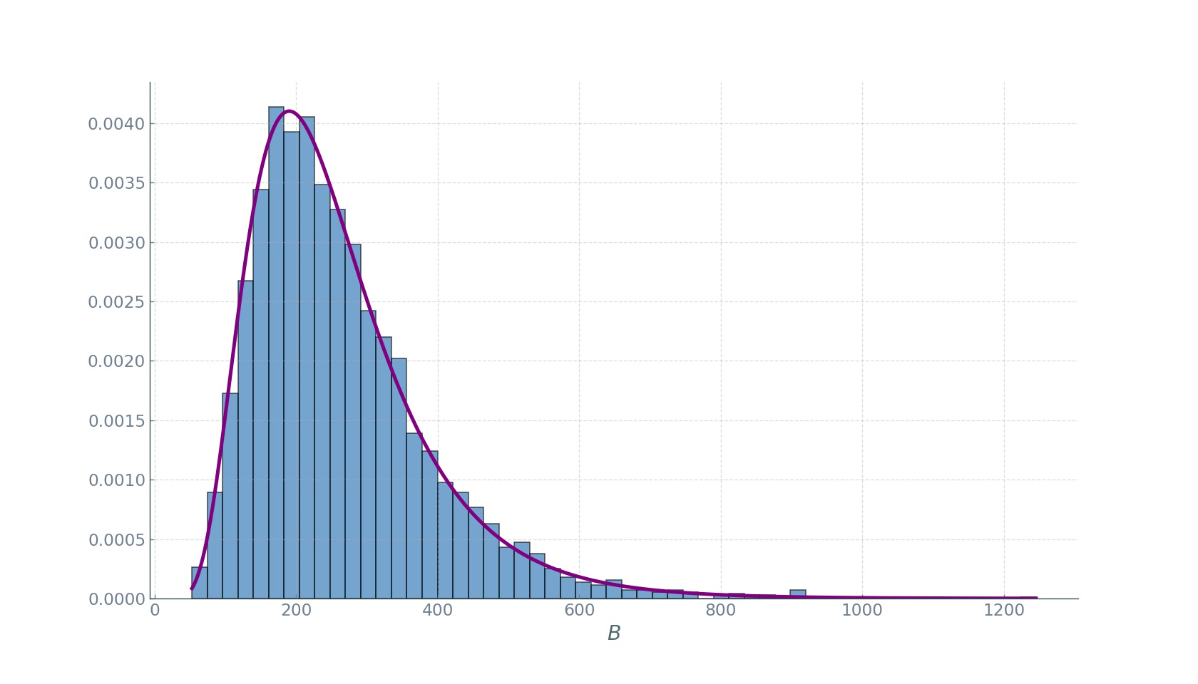
Now, in the expression for \(\langle C\rangle_{N_{T}}\) we simply replace \(\langle L\rangle\) with \(\langle B\rangle\) and obtain our desired \(\langle C\rangle_{N_{V}}\):
\(\langle C\rangle_{N_{V}} \approx 1-\frac{1}{N_{S}} \sum_{i=1}^{N_{S}}\left(1-p_{i}\right)^{\langle B\rangle \star N_{V}}\).
Results
Now that we have the analytical expression for \(\langle C\rangle_{N_{V}}\), we compute it in two ways:
- using the \(p_i\) obtained from the data
- using the \(p_i\) obtained from the taxi-drive simulation
Finally, we plot them against \(N_{V}\):
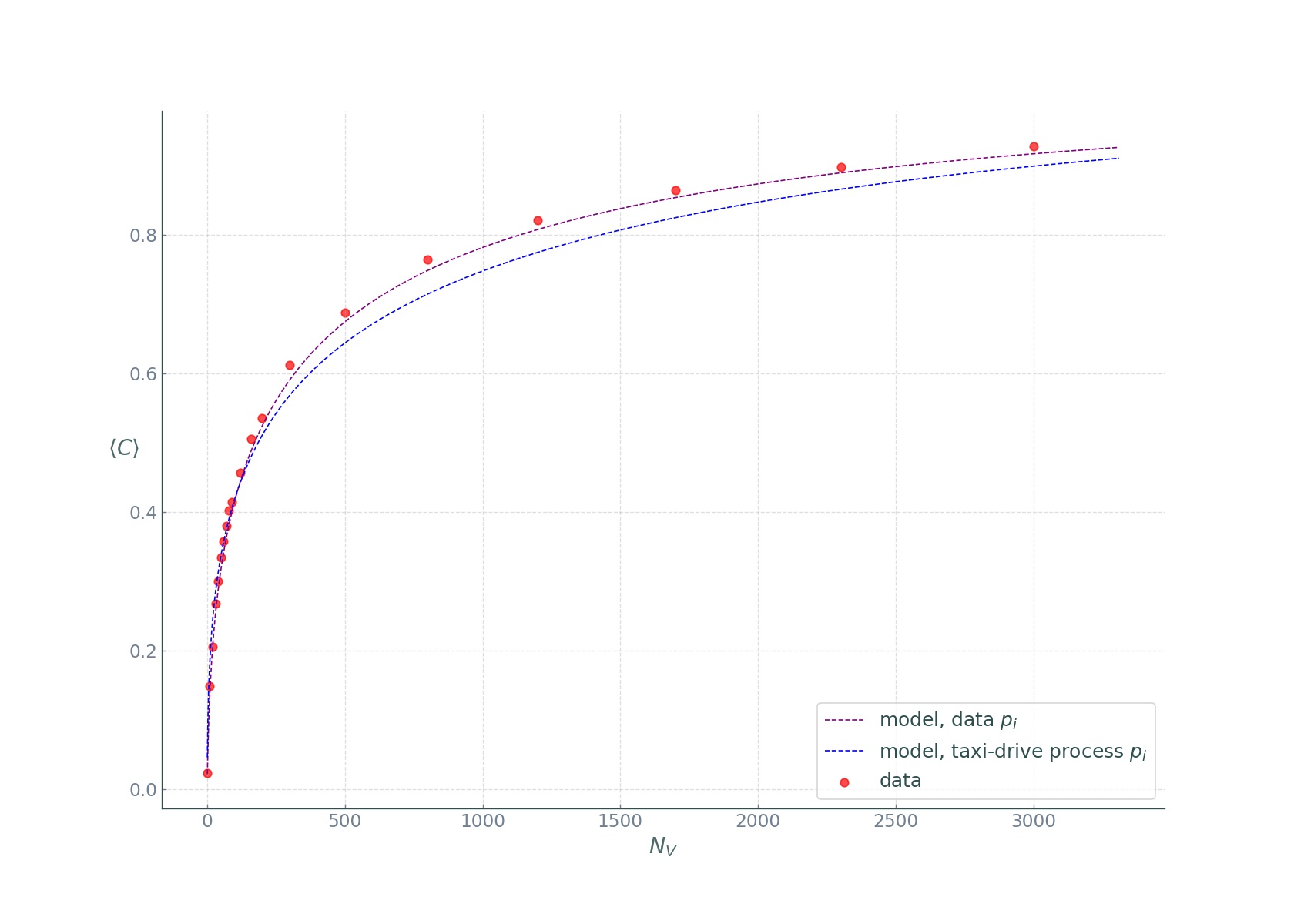
We see that the covered fraction computed the first way is in near perfect agreement with the data, while the second way, despite the oversimplified assumptions, produced impressive results! The rapid increase of the \(\langle C\rangle_{N_{V}}\) curves reveals that taxi fleets have large sensing power, easily covering the popular street segments, while rarely visited unpopular segments, are more and more difficult to cover. We see a law of diminishing returns: while covering the entire city is difficult, a considerable fraction can be covered with relative ease at a low cost. As mentioned in the beginning, only roughly about 30 taxi vehicles are needed to cover more than a third of the entire city, and up to 70% if we restrict the city to the central districts.
Here is a nice animation summarizing the study in Yerevan:
Conclusion
Of course there are many implicit assumptions and scenarios not considered in this study. For instance, we considered \(\mathcal{T}\) to be one day, that is a segment is considered as covered if it is covered at least once by a vehicle from \(\mathcal{V}\) during one day. This is for many sensing purposes too coarse a temporal resolution. For a discussion of finer temporal resolutions, feel free to read the original study. Further, since taxis are concentrated in commercial and touristic neighbourhoods, taxi-based urban sensing displays an inherent spatial bias. This bias could have negative effects, such as underscanning socioeconomically disadvantaged neighborhoods. To overcome this, a hybrid approach to sensing could be attempted. Further yet, our analysis has focused on the fraction of raw segments covered: \(C=\sum 1_{\left(M_{i} \geq 1\right)}\). A more accurate approach would have been to consider the lengths \(b_i\) of the road segments: \(C=\sum b_{i} 1_{\left(M_{i} \geq 1\right)}\).
Despite these and other shortcomings, this work has shown the great potential of taxi-based urban sensing. It will furnish urban practitioners with large amounts of useful data and make possible the development of effective monitoring tools. We have revealed this to be possible with a surprisingly small numbers of sensors.