Medieval urbanism: lessons for contemporary cities

How do cities grow?

Whether large cities are just scaled-up versions of small cities is still an open question. An important one for that matter. In order to plan better cities, we need an improved understanding of how geography, urban economy, social and physical networks and political institutions come together to bring about growth or decline of cities. To achieve this, a thorough outlook on how urban settlements evolved over time is required. Substantial research claims that the social, economic, political, and organizational structures and their innovations that would triumph in “modernity,” “capitalism,” and the Industrial Revolution are rooted in and developed from medieval European settlements. On the other hand, medieval cities were qualitatively different: much smaller, agrarian, with a lower productivity, simpler technologies, and no organized market economy. Strictly hierarchical institutions as the feudal government, Church, and guilds exerted a much stronger influence on the organization of social and economic life in medieval cities compared to analogous structures in modern cities. This influence manifested itself in segregated, corporate societies in which social groupings limited social and economic interactions and opportunities for individuals and families. The modern Western “free flow” of ideas, people, and goods was alien to medieval cities.

These two different and at first sight conflicting perspectives raise the empirical question: Were medieval cities fundamentally different from modern cities? Or is there a continuum of urban processes, form and function from medieval to modern cities?

Far from being just an interesting question, asking such questions is important for building a broad, historically-informed theory of urbanization. In this post, we will narrow down the raised questions and will try to find out whether hierarchical institutions such as the Church or guilds limited and constrained social mixing and interaction in cities affecting urban economic and spatial growth. We will look at a dataset of built-up area and resident populations of 173 medieval cities at circa. 1300 AD, uncover their relationship with simple statistical techniques, and interpret the results in relation to two models from settlement scaling theory. The first model, originally developed for describing modern cities, constructs the built-up area of cities as a function of their population size, considering the city as an unconstrained non-hierarchical socio-economic network embedded in space. The second model builds on top of the first model by adding restrictions to social and economic interactions due to the impact of medieval institutions on social networking. This latter model predicts that, if this restrictive impact is strong, cities will have weak agglomeration effects, which would be visible in the relationship between built-up area and population.

Spatial and social organisation models in cities

On the one hand, one can imagine a medieval city as a self-organized, non-hierarchical social and spatial network entity. If so, interactions among people are only limited by transaction, transportation, opportunity costs, and the so-called “matching costs” of between the needs, skills, and resources of individuals. In such a network, interactions between any two persons are not restricted and occur freely. We will call this view of cities the social reactor model. However, as already mentioned, such hierarchically organized medieval institutions as the Church, feudal authorities, guilds, family ties, etc., exerted huge power and control in medieval cities. This forms the basis for the hypothesis that these institutions strongly regulated the contacts between people in different social groups, hence restricting the social interactions that boost economic productivity, flows of ideas, and the creation of knowledge and innovation. We shall call this view of cities the structured social interaction model and discuss the corresponding mathematical model based on hierarchical graphs capturing the mentioned social and economic regulation. We will then statistically analyse the available data and test our hypothesis by interpreting the results of the data analysis from the perspective of these models.

The Social Reactor Model

The fundamental idea behind most urban socioeconomic theories, including classical models of geography and urban planning, is the concept of a “spatial equilibrium”. In its simplest form formulated by William Alonso, it states that within a city, individuals and firms choose their location by drawing a balance between land rents and transportation costs and economic preferences, given the available resources. This typically leads to a monocentric spatial organisation with the highest land prices at the city core - the most favourable location in terms of accessibility and low transportation costs - decreasing as one moves away from the city center. Urban or settlement scaling theory, on the other hand, has the same basic elements as the Alonso model, except that it offers a more refined modelling framework relating the microprocesses and physical structures in cities to their population through a scaling exponent, as described in what follows. The core idea behind settlement scaling theory is that all human settlements — irrespective of scale or socio-economic complexity — share essential quantitative similarities in terms of general form and function. This comes from the multilayered gains from social agglomeration, whether for economic specialization, innovation, shared infrastructure, common pool of workforce, defence, religion, or trade. In their essence, they model the relationship between various socio-economic characteristics of a city to its population. A key difference between urban economics models and urban scaling theory is the replacement of production or utility functions common in economics with a socio-economic network of interactions.

That said, let’s derive the expected relationship between the population of a city, \(N\), and its built-up area, \(A\). Unlike classical urban economic models, we do not have to assume a radial monocentric city structure. To do this, we balance the average benefit to an individual from social-economic interactions against the associated transportation costs:

\[\frac{GN}{A} = \epsilon A^{\frac{H}{2}}.\]

In the equation, \(G\) is the net benefit per interaction times the area an individual covers over time. Given the differences in social relationships, economic productivity, and innovation in medieval vs. modern cities, \(G\) can vary significantly across time. \(\epsilon\) is the cost of movement per unit length, which is a function of technology (walking, horse riding, etc.). \(H\), another ingredient in specifying the cost associated to individual interactions in a city, is a fractal dimension characterising how people explore a city. For \(H=1\), individuals move in the city through line-like trajectories, while for \(H \rightarrow 2\), they explore the city as an area, exhaustively. In the opposite limit of \(H \rightarrow 0\), individuals remain constrained to a single place (the trajectory is a static point), and the city effectively ceases to be a socio-economic network of interactions. With some simple high school algebra tweaking, we obtain:

\[GN = \epsilon A^{\frac{H+2}{2}}, \ A^{\frac{H+2}{2}} = \frac{G}{\epsilon}N, \ A = aN^\alpha,\]

where \(\alpha := \frac{2}{H+2}\) and \(a := (\frac{G}{\epsilon})^\alpha\). This simple result describes some of the most important properties of urban settlements. First, if benefits from social interactions are small relative to transportation costs, which was the case in medieval cities, then the prefactor, \(a\), will be small and the city will be quite dense. Note also that if \(H = 0\), as could have happened in a segregated settlement, the total built-up area, \(A\), becomes proportional to population, with no agglomeration effects whatsoever. For \(H = 1\), one obtains the special exponent value, \(\alpha = 2/3\), a situation described as the amorphous settlement model, because it neglects any spatial structure and organisation in cities. In such settlements, population density, \(n\), increases rapidly with population size as \(n(N)=\frac{N}{A(N)}=a^{-1} N^{1 / 3}\).

However, so far, we have not yet considered the fact that urban settlements are not organised as blank isotropic canvases, but become organised by locations of interest and the networks making the access to them possible (streets, canals, paths). This means that the effective space for social-economic interactions in cities is defined by its access network. The total network area, \(A_n\), can be derived from population density \(N/A\):

\(A_{n}(N) \sim Nd = A^{1/2}N^{1/2}\) where \(d\) is the average distance between individuals \(d = (A/N)^{1/2}\). Further,

\[A_{n} = l a^{1/2} N^{\alpha/2} N^{1/2} = l a^{1/2} N^{\frac{\alpha + 1}{2}} = a_{0} N^{1-\delta},\]

where \(\delta=\frac{H}{2(H+2)}\) and \(a_{0}=l a^{1 / 2}\). Here \(l\) is a length scale capturing the width of the network at each location of interest (e.g., doors and entrance-ways). For \(H = 1\), we obtain an exponent of \(1-\delta=5/6\).

For the remaining analysis, two aspects of the social reactor model are of particular interest. First, the model predicts that the built-up area of a city should increase with its population, on average, with an exponent \(\frac{2}{3} \leq \alpha \leq \frac{5}{6}\), where the lower bound of 2/3 corresponds to an amorphous isotropic elements, typically small towns, while the upper bound of 5/6 to the role and fine measurement of physical infrastructures in a city. The second aspect has to do with the hierarchical institutions regulating social interactions, and which we will turn our attention to next.

The Structured Social Interaction Model

Now, let’s see how political institutions and social groups can introduce further constraints in social and economic interactions among individuals in cities, and how their influence can change the scaling laws described in the previous section. What we will essentially do is to build a model that moves away from complete freedom with full social mixing in cities towards hierarchical structures of segregated social groups that reduce free social interactions between those groups. These structures can be both formal, such as guilds, parishes, and informal, such as family ties or ethnicity.

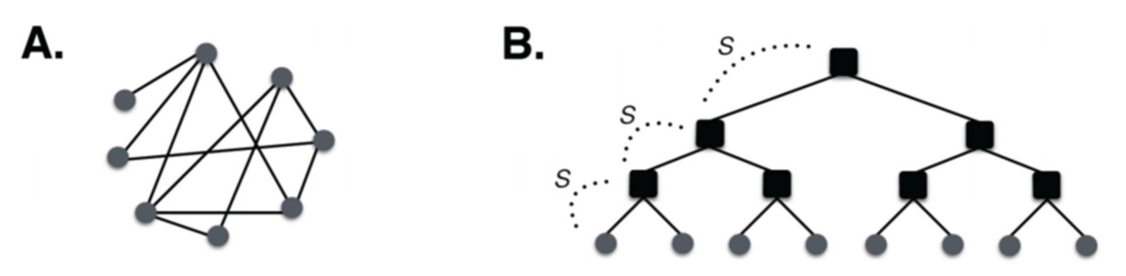
In the image above, A shows an unstructured social network where anyone is free to connect with anyone else, the only limitation being cost of movement. Such a network structure means that connectivity increases rapidly with city population size, with a mean degree of \(k(N)=k_{0} N^{\delta}, \delta \sim 1 / 6\). Conversely, B shows a structured socioeconomic network in which social interactions are regulated by social groups and political institutions (black squares) and, at each level of the hierarchy, may be damped by a factor s<1. This means that the further in hierarchy the connection to another individual is, the more the positive effects of the social interactions will be reduced by dampening them at each level. When s<1, the overall effect of hierarchical institutions is to reduce social possibilities and hence reduce agglomeration effects, forcing the exponent of area scaling with population closer to one.

In fact, the hierarchical structures can also be modelled as contributing to social interaction by reducing interaction costs, for example, by reducing crime or by acting as central places, fostering innovation, such as universities in modern cities. But this is a different story and we will not discuss it here.

The hierarchical structure in the above figure B is parameterized by \(h\) levels and at each level we assume that \(b\) connections are possible, similar to the branching factor in tree graphs. The relationship between \(b\) and the city population, \(N\), is then given by \(h(N)=\log_{b} N\).

We can now derive the number of interactions an individual can have as its contacts are mediated by higher-level groups or social institutions. The important parameter here is the social horizon, \(r=sb\). If \(r>1\), or the effective contact rate, is above one, then the city does not fall apart as a socio-economic network of interactions. For \(r<1\), the city falls apart into distinct groups dictated by the respective institutions.

We begin by considering the number of connections of a typical person. At the first level of the hierarchy, there are \(b\) possible connections, at the second there are \(b+ sb\), at the third \(b+sb+(sb)^2\) and so on. Then, the total number of interactions of a person, at a given level of dampening, \(s\), is the sum of the finite geometric series

\[k_{s}(N)=b\left[1+s b+(s b)^{2}+\ldots\right]=b \frac{1-r^{h}}{1-r}.\]

If you don’t remember this from your high school algebra class, you can find a refresher in the Appendix below. For very small \(s\), we have \(r<<1\) and \(k_{s}(N)=b /(1-s b) \cong b\), which means that all interactions stay essentially limited to the households and there is no city as a network of socio-economic relations at all! In contrast, for \(s\) close to 1, we have \(r>1\), and we can write:

\[k_s(N) = b\frac{(sb)^{h}-1}{sb -1} \approx s^{h}b^h = s^{h}N.\]

Since the city population, \(N\), is proportional to the total infrastructure network area, \(A_n\) times the average connectivity of a typical person, \(k_s(N)\), and since \(h = \log_{b} N\), we obtain

\[A_n \sim \frac{N}{k_s(N)} = s^{-h} = s^{- \log_{b} N} = N^{- \log_{b} s} = N^{\theta},\]

where \(\theta=\left|\frac{\ln s}{\ln b}\right|\). Notice that as \(s \rightarrow 1\), the exponent \(\theta\) goes to zero, rendering the social grouping influence irrelevant. We remember also that as city productivity is proportional to its connectivity, \(A_n = a_0N^{1-\delta} \sim N^{1-\delta}\), and we thus obtain

\[A_n \sim N^{1-\delta + \theta}.\]

In the opposite limit, when social institutions are overly restrictive, we get \(A_n \sim N\), resulting in no population densification (\(n\) = constant) as the city grows. This shows how hierarchical institutions that restrict social opportunities reduce and might even eliminate socio-economic agglomeration effects, spatial densification, and, by implication, cities themselves. Bottom line: If we observe linear scaling of built-up area with population in any urban system, we can identify a situation in which socio-economic restrictions by formal or informal hierarchical institutions could be at play.

Statistical data analysis of medieval urban data

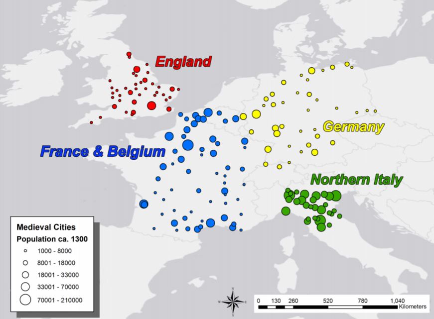
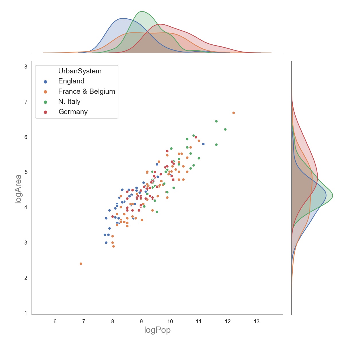
A bit of theory under our belt, let’s uncover statistical relations between urban built-up area and population in a dataset of 173 urban settlements in four different political “urban systems”: Germany, Northern Italy, France & Belgium, and England:

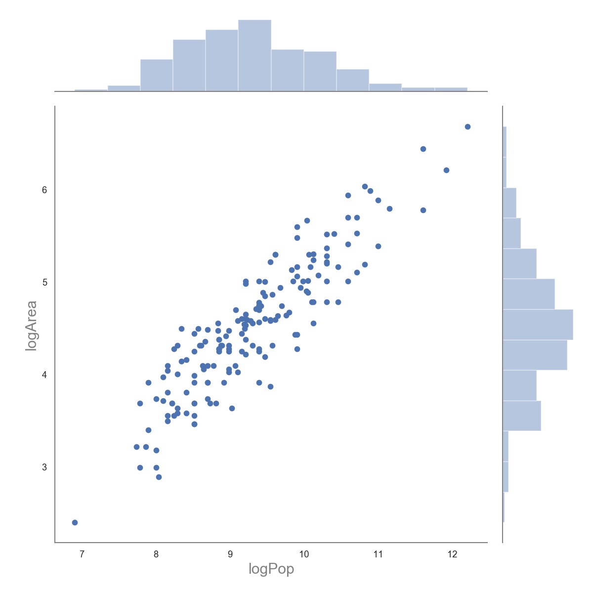
Let’s plot built-up area vs. population for all cities in the dataset to begin with:

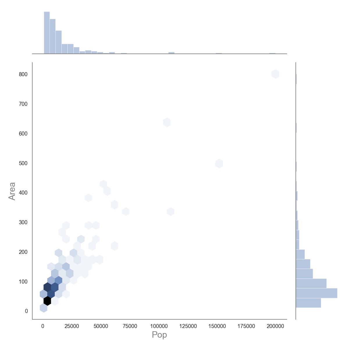
As is typical for city size, we see highly skewed distributions for both area and population. Since a reasonable assumption is that both population and built-up area can’t be too large, we can safely transform the data by taking the natural logarithm of both variables thus “normalising” them and not running the risk of biased regression results because of the fat tails.

Much better! Since the four geopolitical groups could have had different socio-economic structures, we ought to control for them. Let’s break the plot down by the urban system:

Now, we essentially define the following ordinary least squares model:

\[\ln \left(\operatorname{area}_{i}\right)=\alpha+\beta \ln \left(\text {population}_{i}\right)+\epsilon,\]

where \(i\) is the index of a city within a specified urban system and \(\epsilon\) denotes i.i.d. Gaussian distributed error. Note that this is simply a log-transformed version of the social reactor model discussed above, and that \(\beta\) is the same as the scaling coefficient \(\alpha\) in the original model. Having the data prepared, let’s first run the model for all cities together. Here are the regression results:

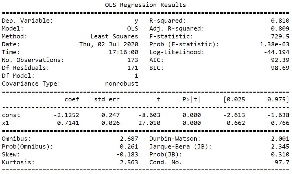
We see that the estimated parameter of interest, the scaling coefficient, \(\beta\), is 0.714, which lies between 2/3 and 5/6! This is a first hint that the statistical distributions of population and area of medieval cities are in acceptable agreement with urban scaling theory. Before we move on, let’s first run some diagnostic tests, to make sure we don’t have heteroskedasticity or normality issues. We can begin with the residual plot:

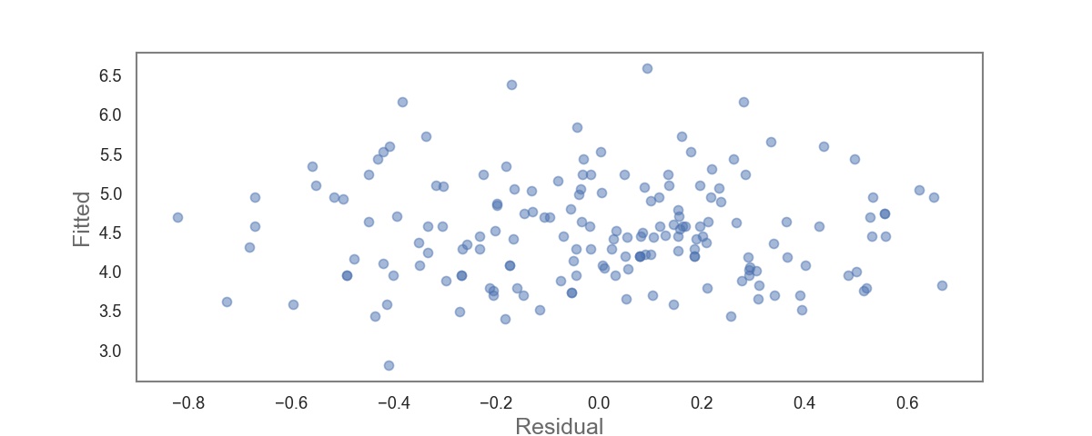
Good, it looks fairly random. For heteroskedasticity, a situation in which the variance of the error term is not the same across observations, we will use the Breusch-Pagan test which is essentially a chi-squared test. Skipping the maths, what matters is that if we obtain a small p-value (<0.05), it’s an indication that we have heteroskedasticity and that it should be addressed. Luckily, we obtain a p-value of 0.644, so we can safely assume homoskedasticity.

To check for normality, we look at the Q-Q plot:

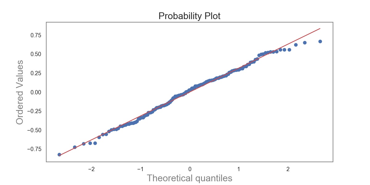
and see a remarkably good agreement with the normality assumption.

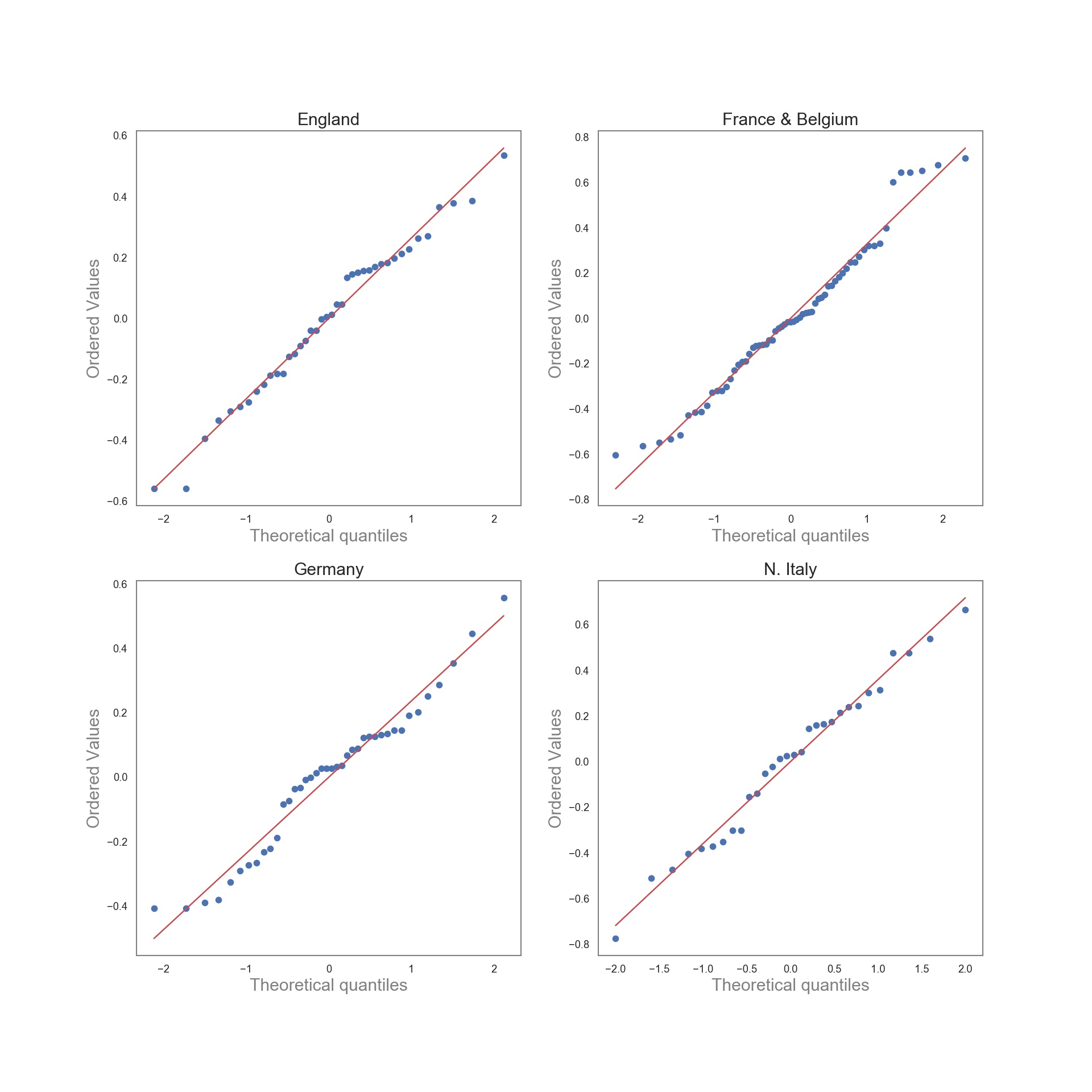
Let’s now move on to running four different models, one for each geopolitical urban system. All p-values obtained from the Breusch-Pagan tests for the four urban systems are much larger than 0.05 and the Q-Q plots for all four models are shown below:

With no violations of our regression assumptions, we plot the regression lines in log space for the four urban systems:

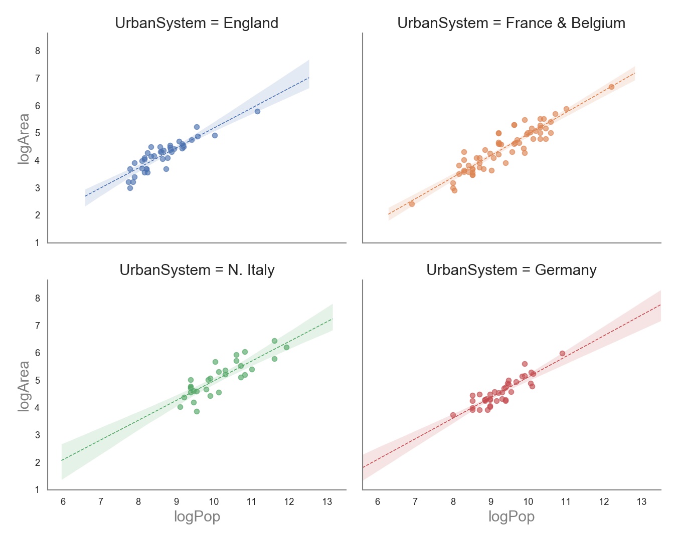
The estimated scaling coefficients are

• England: 0.73
• France & Belgium: 0.79
• Germany: 0.75
• Northern Italy: 0.72

Even with the confidence intervals taken into account, the estimated scaling coefficients are quite similar across geopolitical urban systems with \(2 / 3 \leq \alpha \leq 5 / 6\) as predicted by the social reactor model, and none of the coefficients are \(\geq 5 / 6.\) For this reason, we cannot detect statistically significant evidence that hierarchical institutions limit socio-economic interactions in medieval cities. Of course, since the coefficients fall roughly in the middle of the \(2 / 3 \leq \alpha \leq 5 / 6\) range, some socio-economic dampening might still have occurred. Nonetheless, the consistent estimated scaling coefficients fall well close to those of modern cities and were not dampened towards one. This suggests that the hierarchical institutions of medieval cities did not have a visibly restrictive influence on urban socio-economic interactions, at least within the framework predicted by the structured interactions model.

Conclusion

Despite many structural, social and economic differences, medieval urban settlements have at least one basic property in common with modern cities: larger cities are denser than smaller cities within a given urban system. Overall, the data showed us that city areas did not grow with population faster than what the social reactor or structured interaction models would predict, suggesting that no evidence for restrictive dampening of socio-economomic connectivity and agglomeration effects in medieval cities. Despite the hierarchical institutions prevalent in medieval cities, and which are seemingly not so dominant in Western cities today, we can interpret this result as rejecting the intuitive idea of a strongly segregating role of medieval social institutions. This means that the hierarchical institutions of Western European cities ca. 1300 AD did not considerably restrict social mixing, economic integration, or the free flow of people, ideas, and information. These findings indicate that at a basic structural level, the micro-level socio-economic processes of medieval cities were fundamentally similar to those of modern cities. Even though there are many structural, functional, and cultural differences, both medieval and contemporary cities seem to be described by social networks that become increasingly denser in space as they grow. All this suggests that past cities can be better understood through modern urbanism, but also that modern cities can be better understood by medieval or perhaps even ancient urbanism. With increasing quantity and quality of historical data, we can expect this to be the case.

The jupyter notebook with the code for this post can be found here.

Appendix

For \(r \neq 1,\) the sum of the first \(n\) terms of a geometric series is

\[a+a r+a r^{2}+a r^{3}+\cdots+a r^{n-1}=\sum_{k=0}^{n-1} a r^{k}=a\left(\frac{1-r^{n}}{1-r}\right),\]

where \(a\) is the first term of the series, and \(r\) is the common ratio. We can derive the formula for the sum, \(s\), as follows:

\[\begin{aligned} s &=a+a r+a r^{2}+a r^{3}+\cdots+a r^{n-1} \\ r s &=a r+a r^{2}+a r^{3}+\cdots+a r^{n-1}+a r^{n} \\ s-r s &=a-a r^{n} \\ s(1-r) &=a\left(1-r^{n}\right) \\ s &=a\left(\frac{1-r^{n}}{1-r}\right) \quad(\text { if } r \neq 1) \end{aligned}\]