Why correlation can tell us nothing about outperformance

Introduction

We often hear claims along the lines of “there is a correlation between x and y”. This is especially true with alleged findings about human or social behaviour in psychology or the social sciences. A reported Pearson correlation coefficient of 0.8 indeed seems high in many cases and escapes our critical evaluation of its real meaning.

So let’s see what correlation actually means and if it really conveys the information we often believe it does.

Inspired by the funny spurious correlation project as well as Nassim Taleb’s medium post and Twitter rants in which he laments psychologists’ (and not only) total ignorance and misuse of probability and statistics, I decided to reproduce his note on how much information the correlation coefficient conveys under the Gaussian distribution.

Bivariate Normal Distribution

Let’s say we have two standard normally distributed variables $X$ and $Y$ with covariance structure

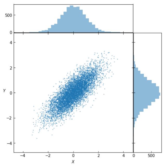
\[\Sigma =\left[\begin{array}{cc}{1} & {0.8} \\ {0.8} & {1} \end{array}\right]\]

Due to the variables being standard normal, the correlation is \(\rho= 0.8\). If we hear someone reporting this correlation between, say, IQ and “success” (whatever it means), it would probably sound convincing.

Let’s visualise the bivariate distribution of \(X\) and \(Y\):

Proportion of uncertainty

In order to understand what the correlation tells us at different intervals of the domain of the data distribution, let’s consider the ratio of the probability of both $X$ and $Y$ exceeding a threshold $K$ under a correlation structure $\rho$, over the probability of both \(X\) and \(Y\) exceeding this threshold given \(\rho=1\). Let’s call this ratio the “proportion of uncertainty”:

\[\phi(\rho, K)=\frac{P\left.(X>K, Y>K)\right|_{\rho}}{P\left.(X>K, Y>K)\right|_{\rho=1}}=\frac{P(X>K, Y>K)}{P(X>K)}\]

Before moving on to evaluate \(\phi(\rho, K)\), let’s first take a look at what the threshold \(K\) represents:

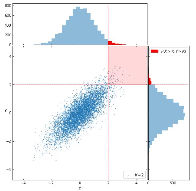
In the image above, \(K=2\), and the shaded region represents the subset of the sample space for which both \(X > K\) and \(Y > K\).

In order to evaluate \(\phi(\rho, K)\), we notice that the joint probability

\[P(X>K, Y>K) = \int_{K}^{\infty}\left(\int_{K}^{\infty} \frac{e^{-\frac{x^{2}+y^{2}-2 x y \rho}{2\left(1-\rho^{2}\right)}}}{2 \pi \sqrt{1-\rho^{2}}} d x\right) d y\]

is impossible to integrate analytically, so we have to resort to numerical computation. Let’s see how we can do it in python.

import numpy as np
from scipy.stats import norm
from scipy.stats import mvn
def phi_func(rho, K):
    
    '''Here we define the phi as a function of rho and K'''
    
    # construct an array of covariance matrices for each rho
    COV = np.array([[
            [1, r],
            [r, 1]] for r in rho]) 
    
    # scipy doesn't offer a survival function (i.e. complementary cdf), so we have to build it  
    threshold = np.array([K, K])
    upper = np.array([100, 100])
    nom_phi = np.array([mvn.mvnun(threshold,upper,mean,cov)[0] for cov in COV])
    
    return nom_phi/(1 - norm.cdf(K))

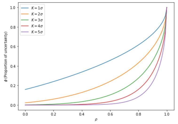
Having \(\phi(\rho, K)\), we plot it against \(\rho\), and obtain:

Conclusion

What we can see from the plot is that the information conveyed by the correlation between \(X\) and \(Y\) behaves disproportianately. From a practical point of view, this means that a correlation of 0.5, for instance, carries very little information (\(\phi\) is somewhere between 0.1 and 0.3) for ordinary values (up to two standard deviations away) and carries essentially no information about the tails (i.e. outliers or outperformers).

Returning to Taleb’s attack on the validity of psychometric tests, the result obtained above means, to quote Taleb, that you need something >.98 to “explain” genius.

The complete Jupyter Notebook with all the code for this post can be found here.