
Jensen’s inequality, decision making under uncertainty, and why economic liberalism inevitably(?) leads to a planned economy
Convex functions
The Covid-19 coronavirus epidemic, as an external shock leading to a global crisis, motivates thinking about our socio-economic system’s capacity to deal with shock events and ask what its inherent structural logic might tell us about the future of the system.
Mathematics, particularly probability theory, apart from its beautiful self-contained world, occasionally offers us incredibly simple yet powerful concepts to help us understand our world.
One such concept is Jensen’s inequality. Imagine a simple function \(f(x) = x^2\) or \(f(x) = e^x\). These are examples of so-called convex functions. In layman’s terms, they “bulge” downwards and demonstrate monotonic growth on both sides. The opposite, bottom-up functions are called concave and “bulge” upwards. Now, imagine \(x\) is a random variable with a certain distribution with finite mean. We know from probability theory that \(f(x)\) is also a random variable, although with a different distribution.
Non-linearity
So what does this have to do with systems containing uncertainty, ranging from natural selection to urban planning and state policy making? If we look around us and take as \(x\) some kind of event intensity, such as deaths from an epidemic or damage from a natural disaster or our being right/wrong on some issue, then \(f(x)\) - the gain/loss from these events - is almost always a non-linear function, either convex or concave.
A few examples to illustrate this: to crush your car 100 times at a speed of 1 km/h is not the same as crushing your car once at the speed of 100 km/h. Every additional speed unit is deadlier than the previous one. Collaboration between humans is also highly convex: 2 + 2 equals much more than 4, and 2 + 2 + 2 equals much much more than 6. This non-linearity of gain underpins the emergence and growth of cities.
So what does this mean? We often hear that many scientific discoveries were made thanks to luck, or serendipity, through trial and error. But this misses the key point: it’s not just trial and error, it’s trial and small error. Luck will systematically favour scientific progress only if the gains from success are progressively more than the losses from error. Otherwise, nobody would do science. The cost of random mutations during evolution were small, it cost close to nothing for some gene to mutate, but the potential gains, that is a species capable of survival, were disproportionately huge!
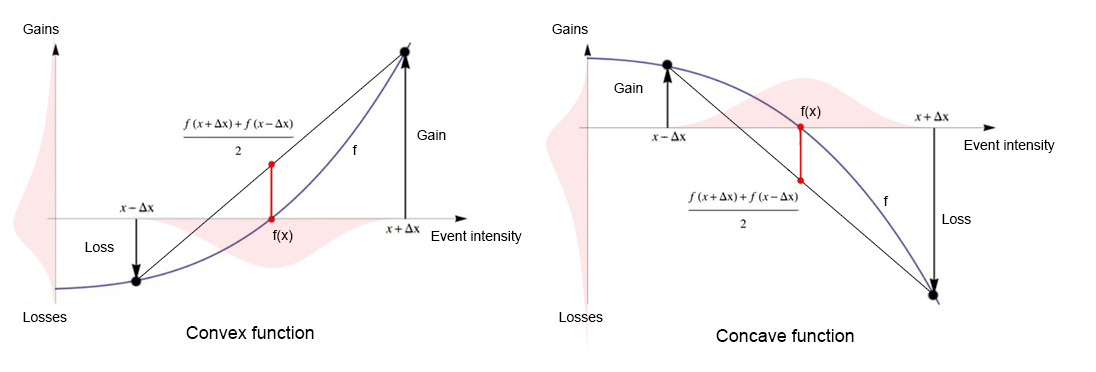
The same is valid for losses: urban planners know very well that if a city saturated with vehicles has, let’s say, 500,000 cars, and the inflow of 10,000 new cars increases average travel time (i.e. the cost) by 5 minutes, then each additional inflow of 10,000 new cars will increase the cost not by 5, but 10, then 20, etc. minutes. This asymmetric nature of gain or loss functions underlies all decision making under uncertainty. You can see it in the diagram below:

Jensen’s inequality
We needed an intro to convex functions to build Jensen’s inequality upon. It is generally stated in the following form: if X is a random variable and \(f\) is a convex function, then
\(f(\mathbf{E}[X]) \leq \mathbf{E}[f(X)]\).
In English, this means that if \(f\) is convex, than under random \(x\)s the average of the function of those \(x\)s is greater or equal to the function of \(x\)’s average. You can see the difference between these two in the image above as the highlighted red line. The same is true for concave functions, albeit with an opposite sign: \(f(\mathbf{E}[X]) \geq \mathbf{E}[f(X)]\).
In real life, this means that if our payoff or gain function is convex, than we benefit from uncertainty. This is because the average gain from the fluctuations of \(x\), i.e. \(\mathbf{E}[f(X)]\) is always greater or equal to the case if we were to prefer certainty and opt for a fixed average value of \(x\) and obtain a gain of \(f(\mathbf{E}[X])\). For example, hospitalized patients from Covid-19 put on lung ventilators are advised to be given random doses of oxygen ranging in the 80-120% of the correct dose. Due to the convexity of the gain to the patient, the average gain from such dose fluctuations is higher than the gain from the correctly specified dose (in the left of the image).
The opposite also holds: given a concave loss function, we should avoid uncertainty. Developing the city traffic example, urban planners should come up with such territorial development and zoning strategies as to minimize the daily fluctuations of car inflow in the city, since the average loss from random car inflow is greater or equal to a more or less certain amount of flow (right of the image).
Liberalism and planned economy
In a simplified setting, economic liberalism and, consequently, liberal ideology, reflected in the support of growing consumer behaviour and individualism, function flawlessly as long as the gain function from the individual, “free” actions of individuals and businesses is convex! That is, as long as the average gain to system from free individual behaviour is greater than the gain from planned, prescribed average behaviour to each individual.
However, as we know from history, an indispensable attribute of economic liberalism are economies of scale as well as production and supply chain optimization to maximise profit. However, economies of scale and overoptimization secretly increase systemic risk by flattening the convex gain functions and turning them into concave loss functions. Now the losses become non-linear to shock events. For example, due to the non-linearity of losses caused by economies of scale and overoptimization, during the past 100 years, the damages from natural disasters such as hurricanes or earthquakes has been growing (as % of GDP) despite unprecedented technological progress.
Under such conditions, when the systemic changes have made the gain functions no more convex, the individuals’ “free” economic, and, consequently, cultural and political actions become a threat to the system. Why?
Let’s say \(J\) is the set of all agents in an economy, and \(P\) is the probability measure assigned to that set, for example, \(P(j)=1 /|J|\) for \(j \in J\). \(X\) is the set of actions each agent must choose from. The set \(S\) lists possible event intensities. The objective function \(f(\cdot, \cdot): X \times S \rightarrow R\) maps actions and events into the real line. Each agent wants to choose an action that maximizes \(f(\cdot, r)\), where \(r \in S\) is the actual event intensity. All agents know that \(r \in S\), but they may not know and may hold different beliefs about the (random) event intensity \(r\). Hence, they may not be able to solve the optimization problem \(\max_{x \in X} f(x, r)\).
Let’s say that a central planner can prescribe each agent a feasible action. Thus, the planner selects any element of the Cartesian product set \(X^{J}\). Let \(\boldsymbol{w} \equiv\left(w_{j}, j \in \boldsymbol{J}\right)\) be any set of assigned actions with finite mean \(\mu_{w} \equiv \int w_{j} d P(j)\). Then, Jensen’s inequality yields
\(f\left(\mu_{w}, s\right) \geq \int f\left(w_{j}, s\right) d P(j) \quad \text { for all } s \in S\).
As we can see, the average payoff when the planner assigns every agent action \(\mu_{w}\) is greater or equal to the payoff with the diversified assignments \(\left(w_{j}, j \in J\right)\).
In other words, Jensen’s inequality tells us that under concave loss functions, the average systemic loss from many individual, different actions is greater than the loss in a planned economy setting with economic action prescribed to each individual!
Structural change
Thus, inherently caused structural changes in liberal economies lead to concave loss functions and thus start favouring tools from a planned economy to manage risk and growth in such a setting. We have witnessed such back and forth transitions from free trade to protectionism and back many times throughout history: from the protectionist politics of Henry VII banning raw wool exports to boost domestic wool cloth production in 15th century England, or from the famous “corn laws” protecting British farmers from cheap Russian corn, to the forceful rise of South Korean industrial potential with policies borrowed from planned economies by Park Chung-hee, to the protection at all costs of nowadays Russian industries of strategic importance.
As beautifully shown by the economic historian Fernand Braudel, the free market and capitalism are not only not the same thing, as often thought, but that the capitalist world-system has been made possible only through the brute force enforcement by a centralized state power. Braudel calls capitalism contre marche. Afterwards, the planned, centralised system makes the gain function convex again, and recedes, allowing economic liberalism to take over again, in order to expand and “enjoy” the conquered markets.
Although many economists have described similar historic economic cycles (Kondratiev, Arrighi, Braudel), of course, everything is much more complex than what I sketched above, since economic liberalism, political liberalism, and cultural liberalism, in their turn, have non-linear dependencies impossible to formalise mathematically for now.
Following the collapse of the Soviet Union, Francis Fukuyama proclaimed the famous “End of History”, claiming essentially that humanity had found the right socio-political system - liberal democracy - and that it should only be corrected, but is, in principle, right.
The main message and hypothesis of this essay is that economic liberalism inevitably (?) contains the seeds of its own destruction, but also of its renaissance. These phase transitions can happen smoothly, without big global shocks, but may also take place in a catastrophic course of events. Fukuyama recently admitted that he was a bit too quick to declare the end of history. Let’s see.